Notes on Tracking Elongated Particles
A tutorial using convolution based least-squares fitting.
Contents
Introduction
If you are not familiar with convolution based least-squares fitting please see: http://gibbs.engr.ccny.cuny.edu/technical/Tracking/ChiTrack.php.
For elongated particles the angle of the particle is needed to determine the position of the particle. One approach would be to use least-squares fitting with an elongated ideal particle. In that case, if we knew the angle of the particle, the entire fitting process could not be done with a single convolution. If the angle is unknown, then many fits with ideal particles at different angles would need to be calculated.
Here another approach will be taken. The ends of long particles look more like a circle than any other part of the particle. Therefore we can fit with a circle of diameter equal to the minimum of the length and width of the object. This will find the two ends of the particle in one pass. Notes on the procedure follow:
Create image with non-overlapping rectangular particles
20 particles of length L, width W are placed in a NNx X NNy sized image.
L=25;   % length of rectangular particles
W=5;    % width of rectangular particles

NNx=256;  % size of test image
NNy=256;

[xx yy]=ndgrid(-NNx/2:NNx/2-1,-NNy/2:NNy/2-1);  % test image grid

% positions of particles:
[px py]=ndgrid(-NNx/2+NNx/8:NNx/4:NNx/2-NNx/8,-NNy/2+NNy/8:NNy/4:NNy/2-NNy/8);
Np=numel(px);

rng('default'); % initialize rand (demo only)
rng(2);

% add some randomness, but don't let overlap
px=px(:)+L/3*randn(Np,1);
py=py(:)+L/3*randn(Np,1);

th=rand(Np,1)*pi; % angle of particles

% add some trouble makers
px=[px;100; 90;90;70];
py=[py;100;100;70;70];
th=[th;pi/6*[-1;-1;1;1]];

Np=length(px);

im=0;  % blank image
for np=1:Np
  rr=(xx+1i*yy+px(np)+1i*py(np))*exp(-1i*th(np));  % grid for particle np
  im=im+(ipf(real(rr),W,1).*ipf(imag(rr),L,1));    % add image of particle np
end
simage(im);  % image of rectangular particles
title(sprintf('%d %d x %d Rectangular Particles',Np,L,W));

Create Ideal Particle
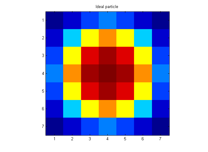
Here an ideal particle of diameter min(L,W) is created.
D=min(L,W);
[x y]=ndgrid(-fix(D/2)-1:fix(D/2)+1,-fix(D/2)-1:fix(D/2)+1); % ideal particle image grid
r=hypot(x,y);

ip=ipf(r,D,1);  % Create ideal particle image

simage(ip);
title('Ideal particle');
Calculate Least-Squares Fit Function
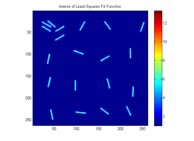
The fit function gives peaks at the ends of each particle.
ichi=1./chiimg(im,ip);  % The inverse of the least-squares fit function is
                        % used since it is easier to see peaks than
                        % valleys.

simage(ichi);
title('Inverse of Least-Squares Fit Function');
colorbar;
Extract End Points
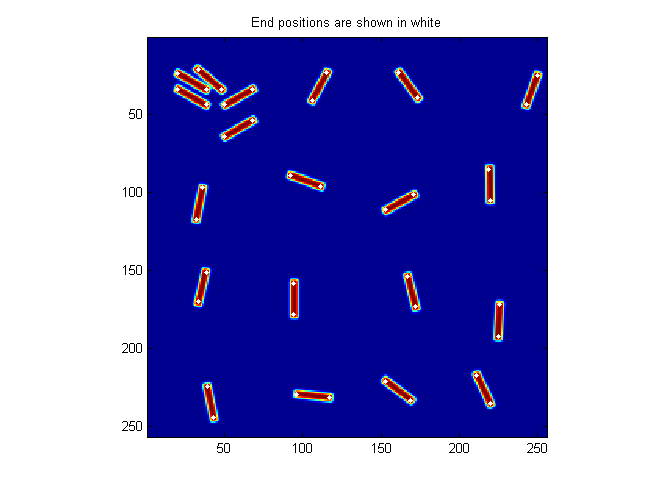
A simple threshold can be used to distinguish the peaks at the ends. In this case 10 works well. The findpeaks function finds 40 ends.
MinSep=L/8;       % minimum separation between peaks
Cutoff=10;        % minimum peak intensity
[Np spx spy]=findpeaks(ichi,1,Cutoff,MinSep);

simage(im);
hold on;
plot(spy-fix(D/2)-1,spx-fix(D/2)-1,'w.');
hold off;
title('End positions are shown in white')
Matching End Points
Matching the ends together to identify the 20 particles could be done in a number of ways depending on data.
m-files
- LongParticleNotes.zip All m-files for tracking tutorials zipped
- LongParticleNotes.m Notes on Tracking Elongated Particles: A tutorial using convolution based least-squares fitting. (This File)
- chiimg.m Calculate chi-squared image.
- findpeaks.m Find intensity peaks in a image
- ipf.m Calculate ideal particle image.
- simage.m Display scaled image.
